In this section, we describe a generalization of
![]() -means, the EM algorithm. It can be applied to a
larger variety of document representations and distributions
than
-means, the EM algorithm. It can be applied to a
larger variety of document representations and distributions
than ![]() -means.
-means.
In ![]() -means, we attempt to find centroids that are good
representatives. We can view the set of
-means, we attempt to find centroids that are good
representatives. We can view the set of ![]() centroids as a model that
generates the data. Generating a document in this model consists of
first picking a centroid at random and then adding some noise. If the
noise is normally distributed, this procedure will result in
clusters of spherical shape.
Model-based clustering
assumes
that the data were generated by a model and tries to
recover the original model from the data. The model that we
recover from the data then
defines clusters and an assignment of documents to clusters.
centroids as a model that
generates the data. Generating a document in this model consists of
first picking a centroid at random and then adding some noise. If the
noise is normally distributed, this procedure will result in
clusters of spherical shape.
Model-based clustering
assumes
that the data were generated by a model and tries to
recover the original model from the data. The model that we
recover from the data then
defines clusters and an assignment of documents to clusters.
A commonly used criterion for estimating the model parameters
is maximum
likelihood. In ![]() -means,
the quantity
-means,
the quantity
![]() is proportional to the
likelihood that a particular model (i.e., a set of centroids) generated
the data. For
is proportional to the
likelihood that a particular model (i.e., a set of centroids) generated
the data. For ![]() -means,
maximum likelihood
and minimal RSS are equivalent criteria.
We denote the model parameters by
-means,
maximum likelihood
and minimal RSS are equivalent criteria.
We denote the model parameters by ![]() .
In
.
In ![]() -means,
-means,
![]() .
.
More generally, the
maximum likelihood criterion is
to select the parameters ![]() that maximize the log-likelihood
of generating the data
that maximize the log-likelihood
of generating the data ![]() :
:
 |
(198) |
This is the same approach we took in Chapter 12
(page 12.1.1 ) for language modeling and in
Section 13.1 (page 13.4 ) for text
classification. In text classification, we chose the class
that maximizes the likelihood of generating a particular
document. Here, we choose the clustering ![]() that
maximizes the likelihood of generating a given set of
documents. Once we have
that
maximizes the likelihood of generating a given set of
documents. Once we have ![]() , we
can compute an assignment probability
, we
can compute an assignment probability
![]() for each document-cluster pair. This
set of assignment probabilities defines a soft clustering.
for each document-cluster pair. This
set of assignment probabilities defines a soft clustering.
An example of a soft assignment is
that
a document about
Chinese cars may have a fractional membership of 0.5 in each of the
two clusters China and automobiles, reflecting the fact
that both topics are pertinent. A hard clustering like
![]() -means cannot
model this simultaneous relevance to two topics.
-means cannot
model this simultaneous relevance to two topics.
Model-based clustering provides a
framework for incorporating our knowledge about a domain.
![]() -means and the
hierarchical algorithms in Chapter 17
make fairly rigid assumptions about the data. For example,
clusters in
-means and the
hierarchical algorithms in Chapter 17
make fairly rigid assumptions about the data. For example,
clusters in ![]() -means are assumed to be spheres.
Model-based clustering offers more flexibility. The
clustering model can be adapted to what we know about the
underlying distribution of the data, be it
Bernoulli (as in
the example in Table 16.3 ), Gaussian with non-spherical variance
(another model that is important
in document clustering) or a member of a different family.
-means are assumed to be spheres.
Model-based clustering offers more flexibility. The
clustering model can be adapted to what we know about the
underlying distribution of the data, be it
Bernoulli (as in
the example in Table 16.3 ), Gaussian with non-spherical variance
(another model that is important
in document clustering) or a member of a different family.
A commonly used algorithm for model-based clustering
is the
Expectation-Maximization algorithm or
EM algorithm .
EM clustering is an iterative algorithm that maximizes
![]() .
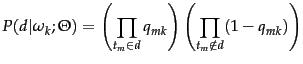
EM can be applied to many different types of probabilistic
modeling.
We will work with a mixture
of multivariate Bernoulli distributions here, the distribution we know from
Section 11.3
(page 11.3 )
and Section 13.3 (page 13.3 ):
.
EM can be applied to many different types of probabilistic
modeling.
We will work with a mixture
of multivariate Bernoulli distributions here, the distribution we know from
Section 11.3
(page 11.3 )
and Section 13.3 (page 13.3 ):
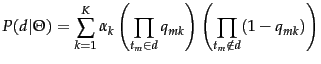
The mixture model then is:
How do we use EM to infer the parameters
of the clustering
from the data? That is, how do we choose parameters ![]() that
maximize
that
maximize
![]() ?
EM is similar to
?
EM is similar to ![]() -means
in that it alternates between an expectation step ,
corresponding to reassignment, and a maximization step ,
corresponding to recomputation of the parameters of the model. The
parameters of
-means
in that it alternates between an expectation step ,
corresponding to reassignment, and a maximization step ,
corresponding to recomputation of the parameters of the model. The
parameters of ![]() -means are the centroids, the parameters of the
instance of EM in this section are the
-means are the centroids, the parameters of the
instance of EM in this section are the ![]() and
and
![]() .
.
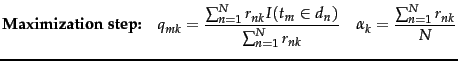
The maximization step
recomputes the conditional parameters
![]() and the priors
and the priors ![]() as follows:
as follows:
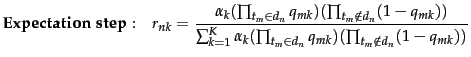
The expectation step computes the soft assignment of
documents to clusters given the current parameters ![]() and
and ![]() :
:
| (a) | docID | document text | docID | document text |
| 1 | hot chocolate cocoa beans | 7 | sweet sugar | |
| 2 | cocoa ghana africa | 8 | sugar cane brazil | |
| 3 | beans harvest ghana | 9 | sweet sugar beet | |
| 4 | cocoa butter | 10 | sweet cake icing | |
| 5 | butter truffles | 11 | cake black forest | |
| 6 | sweet chocolate |
| (b) | Parameter | Iteration of clustering | |||||||
| 0 | 1 | 2 | 3 | 4 | 5 | 15 | 25 | ||
| 0.50 | 0.45 | 0.53 | 0.57 | 0.58 | 0.54 | 0.45 | |||
| 1.00 | 1.00 | 1.00 | 1.00 | 1.00 | 1.00 | 1.00 | |||
| 0.50 | 0.79 | 0.99 | 1.00 | 1.00 | 1.00 | 1.00 | |||
| 0.50 | 0.84 | 1.00 | 1.00 | 1.00 | 1.00 | 1.00 | |||
| 0.50 | 0.75 | 0.94 | 1.00 | 1.00 | 1.00 | 1.00 | |||
| 0.50 | 0.52 | 0.66 | 0.91 | 1.00 | 1.00 | 1.00 | |||
| 1.00 | 1.00 | 1.00 | 1.00 | 1.00 | 1.00 | 0.83 | 0.00 | ||
| 0.00 | 0.00 | 0.00 | 0.00 | 0.00 | 0.00 | 0.00 | 0.00 | ||
| 0.00 | 0.00 | 0.00 | 0.00 | 0.00 | 0.00 | 0.00 | |||
| 0.00 | 0.00 | 0.00 | 0.00 | 0.00 | 0.00 | 0.00 | |||
| 0.50 | 0.40 | 0.14 | 0.01 | 0.00 | 0.00 | 0.00 | |||
| 0.50 | 0.57 | 0.58 | 0.41 | 0.07 | 0.00 | 0.00 | |||
| 0.000 | 0.100 | 0.134 | 0.158 | 0.158 | 0.169 | 0.200 | |||
| 0.000 | 0.083 | 0.042 | 0.001 | 0.000 | 0.000 | 0.000 | |||
| 0.000 | 0.000 | 0.000 | 0.000 | 0.000 | 0.000 | 0.000 | |||
| 0.000 | 0.167 | 0.195 | 0.213 | 0.214 | 0.196 | 0.167 | |||
| 0.000 | 0.400 | 0.432 | 0.465 | 0.474 | 0.508 | 0.600 | |||
| 0.000 | 0.167 | 0.090 | 0.014 | 0.001 | 0.000 | 0.000 | |||
| 0.000 | 0.000 | 0.000 | 0.000 | 0.000 | 0.000 | 0.000 | |||
| 1.000 | 0.500 | 0.585 | 0.640 | 0.642 | 0.589 | 0.500 | |||
| 1.000 | 0.300 | 0.238 | 0.180 | 0.159 | 0.153 | 0.000 | |||
| 1.000 | 0.417 | 0.507 | 0.610 | 0.640 | 0.608 | 0.667 | |||
We clustered a set of 11 documents into two clusters using
EM in Table 16.3 .
After convergence in iteration 25, the first 5 documents are
assigned to cluster 1 (
![]() ) and the last 6 to
cluster 2 (
) and the last 6 to
cluster 2 (![]() ). Somewhat atypically, the final assignment is a hard
assignment here.
EM usually converges to a soft assignment.
In iteration 25, the prior
). Somewhat atypically, the final assignment is a hard
assignment here.
EM usually converges to a soft assignment.
In iteration 25, the prior ![]() for cluster 1 is
for cluster 1 is
![]() because 5 of the 11 documents
are in cluster 1. Some terms are quickly associated with one
cluster because the initial assignment can ``spread'' to them
unambiguously. For example,
membership in cluster 2 spreads
from document 7 to document 8 in the first iteration because they share
sugar (
because 5 of the 11 documents
are in cluster 1. Some terms are quickly associated with one
cluster because the initial assignment can ``spread'' to them
unambiguously. For example,
membership in cluster 2 spreads
from document 7 to document 8 in the first iteration because they share
sugar (![]() in iteration 1).
in iteration 1).
For parameters of terms occurring in
ambiguous contexts, convergence takes longer. Seed
documents 6 and 7 both contain sweet. As a result, it
takes 25 iterations for the term to be unambiguously
associated with cluster 2. (![]() in iteration 25.)
in iteration 25.)
Finding good seeds is even more critical for EM than for
![]() -means. EM is prone to get stuck in local optima if the
seeds are not chosen well. This is a general problem
that also occurs in other applications of EM.
-means. EM is prone to get stuck in local optima if the
seeds are not chosen well. This is a general problem
that also occurs in other applications of EM.![]() Therefore, as with
Therefore, as with ![]() -means, the initial assignment of
documents to clusters is often computed by a different
algorithm. For example, a hard
-means, the initial assignment of
documents to clusters is often computed by a different
algorithm. For example, a hard ![]() -means clustering may
provide the initial assignment, which EM can then ``soften up.''
-means clustering may
provide the initial assignment, which EM can then ``soften up.''
Exercises.