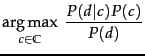
We can interpret
Equation 123 as a description of the
generative process we assume in Bayesian text
classification. To generate a document, we first choose
class ![]() with probability
with probability ![]() (top nodes in
and 13.5 ).
The two models
differ in the formalization of the second step, the
generation of the document given the class, corresponding to
the conditional distribution
(top nodes in
and 13.5 ).
The two models
differ in the formalization of the second step, the
generation of the document given the class, corresponding to
the conditional distribution
![]() :
:
It should now be clearer why we introduced the
document space
![]() in Equation 112 when we defined the classification problem.
A critical step
in solving a text classification problem
is to choose the document
representation.
in Equation 112 when we defined the classification problem.
A critical step
in solving a text classification problem
is to choose the document
representation.
![]() and
and
![]() are two different
document representations.
In the first case,
are two different
document representations.
In the first case,
![]() is the set of all term sequences (or, more
precisely, sequences of term tokens).
In the second case,
is the set of all term sequences (or, more
precisely, sequences of term tokens).
In the second case,
![]() is
is
![]() .
.
We cannot use
and 125 for text
classification directly.
For the Bernoulli model,
we would have to estimate
![]() different
parameters, one for each possible combination of
different
parameters, one for each possible combination of ![]() values
values ![]() and a class. The number of parameters
in the
multinomial case has the same order of
magnitude.
and a class. The number of parameters
in the
multinomial case has the same order of
magnitude.![]() This being a very large
quantity, estimating these parameters reliably is
infeasible.
This being a very large
quantity, estimating these parameters reliably is
infeasible.
To reduce the number of parameters,
we make
the Naive Bayes conditional independence
assumption . We assume that attribute values are independent of
each other given the class:
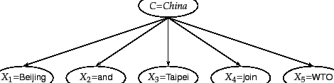
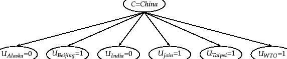
We illustrate the conditional independence assumption in and 13.5 . The class China generates values for each of the five term attributes (multinomial) or six binary attributes (Bernoulli) with a certain probability, independent of the values of the other attributes. The fact that a document in the class China contains the term Taipei does not make it more likely or less likely that it also contains Beijing.
In reality, the conditional independence assumption does not hold for text data. Terms are conditionally dependent on each other. But as we will discuss shortly, NB models perform well despite the conditional independence assumption.
Even when assuming conditional independence, we still have
too many parameters for the multinomial model if
we assume a different probability distribution
for each position ![]() in the
document. The position of a term in a document by itself
does not carry information about the class. Although there is a
difference between China sues France and France
sues China, the occurrence of China in position 1
versus position 3 of the document is not useful in NB
classification because we look at each term separately.
The conditional independence assumption commits
us to this way of processing the evidence.
in the
document. The position of a term in a document by itself
does not carry information about the class. Although there is a
difference between China sues France and France
sues China, the occurrence of China in position 1
versus position 3 of the document is not useful in NB
classification because we look at each term separately.
The conditional independence assumption commits
us to this way of processing the evidence.
Also, if we assumed different term distributions for each
position ![]() , we would have to estimate a different set of
parameters for each
, we would have to estimate a different set of
parameters for each ![]() . The probability of bean
appearing as the first term of a coffee document
could be different from it appearing as the second term, and
so on.
This again causes problems in estimation owing to
data sparseness.
. The probability of bean
appearing as the first term of a coffee document
could be different from it appearing as the second term, and
so on.
This again causes problems in estimation owing to
data sparseness.
For these reasons, we make a second
independence assumption for the multinomial model,
positional independence :
The conditional probabilities for a term are the same
independent of position in the document.
| (128) |
With conditional and positional independence assumptions, we only need to estimate
![]() parameters
parameters
![]() (multinomial model) or
(multinomial model) or
![]() (Bernoulli model), one for each term-class
combination, rather than a number that is at least exponential in
(Bernoulli model), one for each term-class
combination, rather than a number that is at least exponential in
![]() , the size of the vocabulary.
The independence
assumptions reduce the number of parameters to be estimated
by several orders of magnitude.
, the size of the vocabulary.
The independence
assumptions reduce the number of parameters to be estimated
by several orders of magnitude.
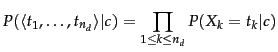
To summarize, we generate a document in the multinomial
model (Figure 13.4 ) by first picking a class ![]() with
with ![]() where
where ![]() is a
random variable taking values
from
is a
random variable taking values
from ![]() as values. Next we generate term
as values. Next we generate term
![]() in position
in position ![]() with
with
![]() for each of the
for each of the ![]() positions of the
document. The
positions of the
document. The ![]() all have the same
distribution over terms for a given
all have the same
distribution over terms for a given ![]() . In the example in
Figure 13.4 , we show the generation
of
. In the example in
Figure 13.4 , we show the generation
of
![]() , corresponding to
the one-sentence document
Beijing and Taipei join WTO.
, corresponding to
the one-sentence document
Beijing and Taipei join WTO.
For a completely specified document generation model, we
would also have to define a distribution
![]() over
lengths. Without it, the multinomial model is
a token generation model rather than a document
generation model.
over
lengths. Without it, the multinomial model is
a token generation model rather than a document
generation model.
We generate a document in the Bernoulli model
(Figure 13.5 ) by first picking a class ![]() with
with
![]() and then generating a binary indicator
and then generating a binary indicator ![]() for
each term
for
each term ![]() of the vocabulary
(
of the vocabulary
(
![]() ).
In the example in
Figure 13.5 , we show the generation
of
).
In the example in
Figure 13.5 , we show the generation
of
![]() , corresponding, again, to the one-sentence document
Beijing and Taipei join WTO where we have
assumed that
and is a stop word.
, corresponding, again, to the one-sentence document
Beijing and Taipei join WTO where we have
assumed that
and is a stop word.
| multinomial model | Bernoulli model | |||
| event model | generation of token | generation of document | ||
| random variable(s) |
|
|||
| document representation |
|
|
||
|
|
||||
| parameter estimation |
|
|
||
| decision rule: maximize |
|
|
||
| multiple occurrences | taken into account | ignored | ||
| length of docs | can handle longer docs | works best for short docs | ||
| # features | can handle more | works best with fewer | ||
| estimate for term the |
|
|
We compare the two models in Table 13.3 , including estimation equations and decision rules.
Naive Bayes is so called because the independence assumptions we have just made are indeed very naive for a model of natural language. The conditional independence assumption states that features are independent of each other given the class. This is hardly ever true for terms in documents. In many cases, the opposite is true. The pairs hong and kong or london and english in Figure 13.7 are examples of highly dependent terms. In addition, the multinomial model makes an assumption of positional independence. The Bernoulli model ignores positions in documents altogether because it only cares about absence or presence. This bag-of-words model discards all information that is communicated by the order of words in natural language sentences. How can NB be a good text classifier when its model of natural language is so oversimplified?
| class selected | |||||
| true probability |
0.6 | 0.4 | |||
|
|
0.00099 | 0.00001 | |||
| NB estimate |
0.99 | 0.01 |
The answer is that
even though the probability estimates of
NB are of low quality, its classification
decisions are surprisingly good. Consider a document ![]() with true probabilities
with true probabilities
![]() and
and
![]() as shown in Table 13.4 .
Assume that
as shown in Table 13.4 .
Assume that ![]() contains
many terms that are positive indicators for
contains
many terms that are positive indicators for ![]() and many terms that are negative indicators for
and many terms that are negative indicators for ![]() .
Thus, when using the
multinomial model in Equation 126,
.
Thus, when using the
multinomial model in Equation 126,
![]() will be much larger than
will be much larger than
![]() (0.00099 vs. 0.00001 in the table).
After division by 0.001 to get well-formed probabilities
for
(0.00099 vs. 0.00001 in the table).
After division by 0.001 to get well-formed probabilities
for ![]() , we end up with one estimate that is close to
1.0 and one that is close to 0.0. This is common:
The winning class in NB classification
usually has a much larger probability than the other
classes and the estimates diverge very significantly from
the true probabilities. But the
classification decision is based on which class gets the
highest score. It does not matter how accurate the
estimates are. Despite the bad estimates, NB
estimates a
higher probability for
, we end up with one estimate that is close to
1.0 and one that is close to 0.0. This is common:
The winning class in NB classification
usually has a much larger probability than the other
classes and the estimates diverge very significantly from
the true probabilities. But the
classification decision is based on which class gets the
highest score. It does not matter how accurate the
estimates are. Despite the bad estimates, NB
estimates a
higher probability for ![]() and therefore assigns
and therefore assigns ![]() to the correct class in Table 13.4 . Correct estimation implies
accurate prediction, but accurate prediction does not imply
correct estimation. NB classifiers estimate badly,
but often classify well.
to the correct class in Table 13.4 . Correct estimation implies
accurate prediction, but accurate prediction does not imply
correct estimation. NB classifiers estimate badly,
but often classify well.
Even if it is not the method with the highest accuracy for text, NB has many virtues that make it a strong contender for text classification. It excels if there are many equally important features that jointly contribute to the classification decision. It is also somewhat robust to noise features (as defined in the next section) and concept drift - the gradual change over time of the concept underlying a class like US president from Bill Clinton to George W. Bush (see Section 13.7 ). Classifiers like kNN knn can be carefully tuned to idiosyncratic properties of a particular time period. This will then hurt them when documents in the following time period have slightly different properties.
The Bernoulli model is particularly robust with respect to concept drift. We will see in Figure 13.8 that it can have decent performance when using fewer than a dozen terms. The most important indicators for a class are less likely to change. Thus, a model that only relies on these features is more likely to maintain a certain level of accuracy in concept drift.
NB's main strength is its efficiency: Training and classification can be accomplished with one pass over the data. Because it combines efficiency with good accuracy it is often used as a baseline in text classification research. It is often the method of choice if (i) squeezing out a few extra percentage points of accuracy is not worth the trouble in a text classification application, (ii) a very large amount of training data is available and there is more to be gained from training on a lot of data than using a better classifier on a smaller training set, or (iii) if its robustness to concept drift can be exploited.
| (1) | He moved from London, Ontario, to London, England. | ||
| (2) | He moved from London, England, to London, Ontario. | ||
| (3) | He moved from England to London, Ontario. |
In this book, we discuss NB as a classifier for text. The independence assumptions do not hold for text. However, it can be shown that NB is an optimal classifier (in the sense of minimal error rate on new data) for data where the independence assumptions do hold.