Next: References and further reading
Up: Postings file compression
Previous: Variable byte codes
Contents
Index
Gamma codes
Table 5.5:
Some examples of unary and  codes.
Unary codes are only shown for the smaller numbers.
Commas in codes are for readability only and are not part of the actual codes.
codes.
Unary codes are only shown for the smaller numbers.
Commas in codes are for readability only and are not part of the actual codes.
| | number |
unary code |
length |
offset |
code |
|
| | 0 |
0 |
|
|
|
|
| | 1 |
10 |
0 |
|
0 |
|
| | 2 |
110 |
10 |
0 |
10,0 |
|
| | 3 |
1110 |
10 |
1 |
10,1 |
|
| | 4 |
11110 |
110 |
00 |
110,00 |
|
| | 9 |
1111111110 |
1110 |
001 |
1110,001 |
|
| | 13 |
|
1110 |
101 |
1110,101 |
|
| | 24 |
|
11110 |
1000 |
11110,1000 |
|
| | 511 |
|
111111110 |
11111111 |
111111110,11111111 |
|
| | 1025 |
|
11111111110 |
0000000001 |
11111111110,0000000001 |
|
VB codes use an adaptive number of bytes
depending on the size of the gap. Bit-level codes adapt the
length of the code on the finer grained bit level.
The simplest bit-level code is unary code . The unary
code of  is a string of 1s followed by a 0 (see the
first two columns of Table 5.5 ).
Obviously,
this is not a very efficient code, but it will come in handy
in a moment.
is a string of 1s followed by a 0 (see the
first two columns of Table 5.5 ).
Obviously,
this is not a very efficient code, but it will come in handy
in a moment.
How efficient can a code be in principle? Assuming the
 gaps
gaps  with
with
 are all equally
likely, the optimal encoding uses bits for each . So
some gaps (
are all equally
likely, the optimal encoding uses bits for each . So
some gaps ( in this case) cannot be encoded with
fewer than
in this case) cannot be encoded with
fewer than  bits. Our goal is to get as close to
this lower bound as possible.
bits. Our goal is to get as close to
this lower bound as possible.
A method that is within a factor of optimal
is encoding .
codes implement variable-length encoding by splitting the
representation of a
gap into a pair of length and offset.
Offset is in binary, but with the leading 1
removed.![[*]](http://nlp.stanford.edu/IR-book/html/icons/footnote.png) For example, for 13 (binary 1101) offset is 101.
Length encodes the length of offset
in unary code.
For 13,
the length of offset is 3 bits, which is 1110 in
unary. The code of 13 is therefore 1110101, the
concatenation of length 1110 and offset 101.
The right hand column of Table 5.5 gives additional
examples of codes.
For example, for 13 (binary 1101) offset is 101.
Length encodes the length of offset
in unary code.
For 13,
the length of offset is 3 bits, which is 1110 in
unary. The code of 13 is therefore 1110101, the
concatenation of length 1110 and offset 101.
The right hand column of Table 5.5 gives additional
examples of codes.
A code is decoded by first reading the unary code
up to the 0 that terminates it, for example, the four bits 1110
when decoding 1110101. Now we know how long the
offset is: 3 bits. The offset 101 can then be read correctly and
the 1 that was chopped off in encoding is prepended: 101
 1101 = 13.
The length of offset is
 bits and the length of length
is
bits and the length of length
is
 bits,
so the length of the entire
code is
bits,
so the length of the entire
code is
 bits. codes are
always of odd length and they are within a factor of
2 of what we claimed to be
the optimal encoding length .
We derived this optimum
from the assumption
that the gaps
between
bits. codes are
always of odd length and they are within a factor of
2 of what we claimed to be
the optimal encoding length .
We derived this optimum
from the assumption
that the gaps
between  and
and  are equiprobable.
But this need not be the case. In general, we do not know the
probability distribution over gaps a priori.
are equiprobable.
But this need not be the case. In general, we do not know the
probability distribution over gaps a priori.
Figure 5.9:
Entropy  as a function of
  for a sample space
with two outcomes
for a sample space
with two outcomes  and
and  .
.
![\includegraphics[width=7cm]{art/entropy.eps}](img293.png) |
The characteristic of a discrete probability
distribution  that
determines its coding properties (including whether a code is
optimal) is its
entropy , which is
defined as follows:
that
determines its coding properties (including whether a code is
optimal) is its
entropy , which is
defined as follows:
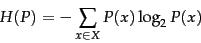 |
(4) |
where  is the set of all possible numbers we need to be
able to encode
(and therefore
is the set of all possible numbers we need to be
able to encode
(and therefore
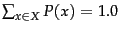 ). Entropy is a
measure of uncertainty as shown in Figure 5.9 for a
probability distribution over two possible outcomes, namely,
). Entropy is a
measure of uncertainty as shown in Figure 5.9 for a
probability distribution over two possible outcomes, namely,
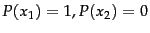
 . Entropy is maximized (
 ) for
) for
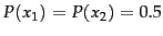 when uncertainty about which
  will appear next is largest; and minimized (
 ) for
) for
 and for
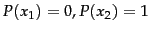 when there is absolute certainty.
It can be shown
that the lower bound for the expected length  of a
code
of a
code  is if certain conditions hold (see the references). It can
further be shown that for
is if certain conditions hold (see the references). It can
further be shown that for
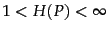 ,
encoding is within a factor of 3 of this optimal encoding,
approaching 2 for large :
,
encoding is within a factor of 3 of this optimal encoding,
approaching 2 for large :
 |
(5) |
What is remarkable about this result is that it holds for
any probability distribution . So without knowing
anything about the properties of the distribution of gaps,
we can apply codes and be certain that they are within a
factor of  of the optimal code for distributions
of large entropy. A code like code with the property of
being within a factor of optimal for an arbitrary distribution is
called
universal .
of the optimal code for distributions
of large entropy. A code like code with the property of
being within a factor of optimal for an arbitrary distribution is
called
universal .
In addition to universality,
codes have two other properties that are useful for index
compression. First, they are
prefix free , namely, no
code is the prefix of another. This means that
there is always a unique decoding of a sequence of
codes - and we do not need delimiters between them,
which would decrease the efficiency of the code. The second
property is that codes are
parameter free . For many other efficient codes, we
have to fit the parameters of a model (e.g., the
binomial distribution) to
the distribution of gaps in the index. This complicates the
implementation of compression and decompression.
For instance, the
parameters need to be stored and retrieved. And in dynamic indexing, the distribution of
gaps can change, so that the original parameters are no longer
appropriate. These problems are avoided with a
parameter-free code.
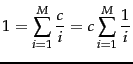
How much compression of the inverted index do codes
achieve? To answer this question we use Zipf's law, the term
distribution model introduced in Section 5.1.2 .
According to Zipf's law, the collection frequency  is proportional to the
inverse of the rank
is proportional to the
inverse of the rank  , that is, there is a constant
  such that:
 |
|
|
(6) |
We can choose a different constant  such that the
fractions
such that the
fractions  are relative
frequencies and sum to 1 (that is,
are relative
frequencies and sum to 1 (that is,
 ):
):
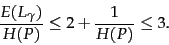
where  is the number of distinct terms and
  is the
th harmonic
number .
Reuters-RCV1 has
is the
th harmonic
number .
Reuters-RCV1 has
 distinct terms
and
distinct terms
and
 , so we have
 |
(9) |
Thus the th term has a relative frequency of roughly
 , and
the expected average number of occurrences of term
in a document of length is:
, and
the expected average number of occurrences of term
in a document of length is:
 |
(10) |
where we interpret the relative frequency as a term occurrence
probability. Recall that 200 is the average number of
tokens per document in Reuters-RCV1 (Table 4.2 ).
Figure 5.10:
Stratification of terms for
estimating the size of a encoded inverted index.
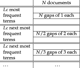 |
Now we have derived term
statistics that characterize the distribution of terms in
the collection and, by extension, the distribution of gaps in
the postings lists.
From these statistics, we can
calculate
the space requirements for an inverted index compressed with
encoding. We first stratify the
vocabulary into blocks of size
 .
On average, term occurs
.
On average, term occurs  times per
document. So the average number of occurrences
times per
document. So the average number of occurrences
 per document
is
per document
is
 for terms in the
first block, corresponding to a total number of
for terms in the
first block, corresponding to a total number of  gaps per
term. The average is
gaps per
term. The average is
 for terms in the
second block, corresponding to
for terms in the
second block, corresponding to  gaps per term, and
 for terms in the
third block, corresponding to
for terms in the
third block, corresponding to  gaps per term, and so on. (We
take the lower bound because it simplifies subsequent calculations.
As we will see, the final estimate is too
pessimistic, even with this assumption.)
We will make the somewhat unrealistic assumption that all
gaps for a given term have the same size
as shown in Figure 5.10.
Assuming such a uniform distribution of gaps,
we then have gaps of size 1 in block 1, gaps of size 2 in
block 2, and so on.
gaps per term, and so on. (We
take the lower bound because it simplifies subsequent calculations.
As we will see, the final estimate is too
pessimistic, even with this assumption.)
We will make the somewhat unrealistic assumption that all
gaps for a given term have the same size
as shown in Figure 5.10.
Assuming such a uniform distribution of gaps,
we then have gaps of size 1 in block 1, gaps of size 2 in
block 2, and so on.
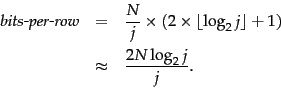
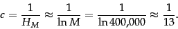
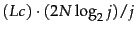
Encoding the  gaps of size
  with codes, the number of
bits needed for the postings list
of a term in the th block (corresponding to one row in
the figure) is:
with codes, the number of
bits needed for the postings list
of a term in the th block (corresponding to one row in
the figure) is:
To encode the entire block, we need
 bits. There are
  blocks, so the postings file as a whole will
take up:
blocks, so the postings file as a whole will
take up:
| |
|
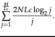 |
(11) |
For Reuters-RCV1,
 400,000
 and
and
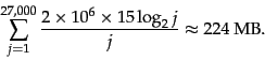 |
(12) |
So the postings file of the compressed inverted index
for our 960 MB collection has a size of 224 MB, one fourth the
size of
the original collection.
When we run compression on Reuters-RCV1,
the actual size of the compressed index is even
lower: 101 MB, a bit more than one tenth of the size of the
collection. The reason for the discrepancy between
predicted and actual value is
that (i) Zipf's law is not a very good
approximation of the actual distribution of term frequencies
for Reuters-RCV1 and (ii) gaps are not uniform. The Zipf model predicts an index size of 251 MB
for the unrounded numbers from Table 4.2 . If
term frequencies are generated from the Zipf model and a
compressed index is created for these artificial terms, then
the compressed size is 254 MB. So to the extent that
the assumptions about the distribution of term frequencies
are accurate,
the predictions of the model are correct.
Table:
Index and dictionary compression for Reuters-RCV1.
The compression ratio depends on the proportion of actual text
in the collection. Reuters-RCV1 contains a
large amount of XML
markup. Using the two best
compression schemes, encoding and blocking with
front coding, the
ratio compressed index to collection size is therefore
especially small for Reuters-RCV1:
 .
.
 .
.
| | data structure |
size in MB |
| | dictionary, fixed-width |
19.211.2 |
| | dictionary, term pointers into string |
10.8 7.6 |
| |  , with blocking, , with blocking,  |
10.3 7.1 |
| | , with blocking & front coding |
7.9 5.9 |
| | collection (text, xml markup etc) |
3600.0 |
| | collection (text) |
960.0 |
| | term incidence matrix |
40,000.0 |
| | postings, uncompressed (32-bit words) |
400.0 |
| | postings, uncompressed (20 bits) |
250.0 |
| | postings, variable byte encoded |
116.0 |
| | postings, encoded |
101.0 |
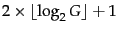
Table 5.6 summarizes
the compression techniques covered in this chapter.
The
term incidence matrix
(Figure 1.1 , page 1.1 )
for Reuters-RCV1 has size
 bits or 40 GB.
The numbers were the collection (3600 MB and 960 MB) are for
the encoding of RCV1 of CD, which uses one byte per
character, not Unicode.
bits or 40 GB.
The numbers were the collection (3600 MB and 960 MB) are for
the encoding of RCV1 of CD, which uses one byte per
character, not Unicode.
codes achieve great compression ratios - about
15% better than variable byte codes for Reuters-RCV1. But they
are expensive to decode. This is because many
bit-level operations - shifts and masks - are necessary to
decode a sequence of codes as the boundaries between
codes will usually be somewhere in the middle of a machine
word. As a result, query processing is more expensive for
codes than for variable byte codes.
Whether we choose variable byte or encoding
depends on the characteristics of an application, for example,
on the relative
weights we give to conserving disk space versus maximizing query
response time.
The compression ratio for the index in
Table 5.6 is about 25%: 400 MB
(uncompressed, each posting stored as a 32-bit word) versus 101 MB
() and
116 MB (VB). This shows that both and VB codes meet
the objectives we stated in the beginning of the chapter.
Index compression substantially improves time and space
efficiency of indexes by reducing the amount of disk space needed,
increasing the amount of information that can be kept in
the cache, and speeding up data transfers from disk to memory.
Exercises.
- Compute variable byte codes for the numbers in
Tables 5.3 5.5 .
- Compute variable byte and codes for
the
postings list
 777, 17743, 294068, 31251336
 . Use gaps instead
of docIDs where possible. Write binary codes in 8-bit blocks.
. Use gaps instead
of docIDs where possible. Write binary codes in 8-bit blocks.
-
Consider the postings list
 with a corresponding list of gaps
 .
Assume that the length of the postings list is stored separately, so the system knows when a postings list is complete.
Using variable byte encoding:
(i) What is the largest gap you can encode in 1 byte?
(ii) What is the largest gap you can encode in 2 bytes?
(iii) How many bytes will the above postings list require under this encoding? (Count only space for encoding the sequence of numbers.)
.
Assume that the length of the postings list is stored separately, so the system knows when a postings list is complete.
Using variable byte encoding:
(i) What is the largest gap you can encode in 1 byte?
(ii) What is the largest gap you can encode in 2 bytes?
(iii) How many bytes will the above postings list require under this encoding? (Count only space for encoding the sequence of numbers.)
- A little trick is to notice that a gap cannot be of length 0
and that the stuff left to encode after shifting cannot be
0. Based on these observations:
(i) Suggest a modification to variable byte encoding that
allows you to encode slightly larger gaps in the same amount
of space.
(ii) What is the largest gap you can encode in 1 byte?
(iii) What is the largest gap you can encode in 2 bytes?
(iv) How many bytes will the postings list in Exercise 5.3.2
require under this encoding?
(Count only space for encoding the sequence of numbers.)
- From the following sequence of -coded gaps,
reconstruct first the gap sequence and then the postings
sequence: 1110001110101011111101101111011.
- codes are relatively
inefficient for large numbers (e.g., 1025 in
Table 5.5 ) as they encode the length of the
offset in inefficient unary code.
 codes
differ from codes in that they encode the first
part of the code (length) in code instead of
unary code. The encoding of offset is the
same. For example, the code of 7 is 10,0,11 (again,
we add commas for readability). 10,0 is the code
for length (2 in this case) and the encoding of offset
(11) is unchanged. (i) Compute the codes for the other
numbers in Table 5.5 . For what range of numbers
is the code shorter than the code?
(ii) code beats variable byte code in
Table 5.6 because the index contains stop words and thus
many small gaps. Show that variable byte code is more
compact if larger gaps dominate. (iii) Compare the
compression ratios of code and variable byte code
for a distribution of gaps dominated by large gaps.
codes
differ from codes in that they encode the first
part of the code (length) in code instead of
unary code. The encoding of offset is the
same. For example, the code of 7 is 10,0,11 (again,
we add commas for readability). 10,0 is the code
for length (2 in this case) and the encoding of offset
(11) is unchanged. (i) Compute the codes for the other
numbers in Table 5.5 . For what range of numbers
is the code shorter than the code?
(ii) code beats variable byte code in
Table 5.6 because the index contains stop words and thus
many small gaps. Show that variable byte code is more
compact if larger gaps dominate. (iii) Compare the
compression ratios of code and variable byte code
for a distribution of gaps dominated by large gaps.
- Go through the above calculation of index size and
explicitly state all the approximations that were made to
arrive at Equation 11.
- For a collection of your choosing, determine the number
of documents and terms and the average length of a
document. (i) How large is the inverted index predicted to be by
Equation 11? (ii) Implement an indexer that
creates a -compressed inverted index for the
collection. How large is the actual index? (iii) Implement an
indexer that uses variable byte encoding. How large is the
variable byte encoded index?
Table:
Two gap sequences to be merged in blocked sort-based indexing
| | encoded gap sequence of run 1 |
1110110111111001011111111110100011111001 |
|
| | encoded gap sequence of run 2 |
11111010000111111000100011111110010000011111010101
|
|
- To be able to hold as many postings as possible in
main memory, it is a good idea to compress intermediate
index files during index construction. (i) This makes
merging runs in blocked sort-based indexing more complicated. As an
example, work out the -encoded merged sequence of
the gaps in Table 5.7 . (ii) Index construction is
more space efficient when using compression. Would you also
expect it to be faster?
- (i) Show that the size of the vocabulary is finite
according to Zipf's law and infinite according to Heaps'
law. (ii) Can we derive Heaps' law from Zipf's law?
Next: References and further reading
Up: Postings file compression
Previous: Variable byte codes
Contents
Index
© 2008 Cambridge University Press
This is an automatically generated page. In case of formatting errors you may want to look at the PDF edition of the book.
2009-04-07