 |
(203) |
The motivation for GAAC is that our goal in selecting two
clusters ![]() and
and ![]() as the next merge in HAC
is that the resulting merge cluster
as the next merge in HAC
is that the resulting merge cluster
![]() should be
coherent. To judge the coherence of
should be
coherent. To judge the coherence of ![]() ,
we need to look at all document-document similarities within
,
we need to look at all document-document similarities within ![]() ,
including those that occur within
,
including those that occur within ![]() and those that
occur within
and those that
occur within ![]() .
.
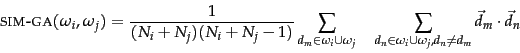
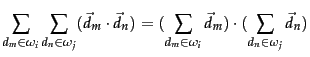
We can compute
the measure SIM-GA
efficiently because the
sum of individual vector similarities is equal to the
similarities of their sums:
Equation 204 relies on the distributivity of the dot product with respect to vector addition. Since this is crucial for the efficient computation of a GAAC clustering, the method cannot be easily applied to representations of documents that are not real-valued vectors. Also, Equation 204 only holds for the dot product. While many algorithms introduced in this book have near-equivalent descriptions in terms of dot product, cosine similarity and Euclidean distance (cf. simdisfigs), Equation 204 can only be expressed using the dot product. This is a fundamental difference between single-link/complete-link clustering and GAAC. The first two only require a square matrix of similarities as input and do not care how these similarities were computed.
To summarize, GAAC requires (i) documents represented as vectors, (ii) length normalization of vectors, so that self-similarities are 1.0, and (iii) the dot product as the measure of similarity between vectors and sums of vectors.
The merge algorithms for GAAC
and complete-link clustering are the same except that we
use
Equation 205
as
similarity function
in
Figure 17.8 . Therefore, the overall time complexity of
GAAC is the same as for complete-link
clustering:
![]() .
Like complete-link clustering, GAAC is
not best-merge persistent
(Exercise 17.10 ).
This means that
there
is no
.
Like complete-link clustering, GAAC is
not best-merge persistent
(Exercise 17.10 ).
This means that
there
is no ![]() algorithm for GAAC
that would be analogous to the
algorithm for GAAC
that would be analogous to the ![]() algorithm
for single-link in Figure 17.9 .
algorithm
for single-link in Figure 17.9 .
We can also define group-average similarity
as including self-similarities:
Self-similarities are always
equal to 1.0, the maximum possible value for length-normalized vectors.
The
proportion of self-similarities in
Equation 206 is ![]() for a cluster of size
for a cluster of size ![]() .
This gives an unfair advantage to small clusters since they
will have proportionally more self-similarities.
For two documents
.
This gives an unfair advantage to small clusters since they
will have proportionally more self-similarities.
For two documents ![]() ,
, ![]() with a similarity
with a similarity ![]() ,
we have
,
we have
![]() . In contrast,
. In contrast,
![]() . This
similarity
. This
similarity
![]() of two documents
is
the same as in single-link,
complete-link and centroid
clustering. We prefer the definition in
Equation 205, which excludes self-similarities
from the average, because we do not want to penalize large
clusters for their smaller proportion of self-similarities
and because we want a consistent similarity value
of two documents
is
the same as in single-link,
complete-link and centroid
clustering. We prefer the definition in
Equation 205, which excludes self-similarities
from the average, because we do not want to penalize large
clusters for their smaller proportion of self-similarities
and because we want a consistent similarity value ![]() for
document pairs in all four HAC algorithms.
for
document pairs in all four HAC algorithms.
Exercises.
![$\displaystyle \frac{1}{(N_i+N_j)(N_i+N_j-1)}[ (\sum_{d_\mthatwask \in
\omega_i \cup \omega_j} \vec{d}_\mthatwask)^2
- (N_i+N_j)]$](img1601.png)
![$\displaystyle \mbox{{\sc sim-ga}}^{\prime}(\omega_i,\omega_j) = \frac{1}{(N_i \...
..._j} \!\!\![\vec{d}_\mthatwask \cdot \vec{\mu} ( \omega_i \! \cup \! \omega_j )]$](img1607.png)