The basic steps in constructing a nonpositional index are
depicted in Figure 1.4 (page ![]() ). We first make a pass
through the collection assembling all
term-docID pairs. We then sort the pairs with the term
as the dominant key and docID as the secondary key. Finally,
we organize the docIDs for each term into a postings list and
compute statistics like term and document frequency. For
small collections, all this can be done in memory. In this
chapter, we describe methods for large collections that
require the use of secondary storage.
). We first make a pass
through the collection assembling all
term-docID pairs. We then sort the pairs with the term
as the dominant key and docID as the secondary key. Finally,
we organize the docIDs for each term into a postings list and
compute statistics like term and document frequency. For
small collections, all this can be done in memory. In this
chapter, we describe methods for large collections that
require the use of secondary storage.
To make index construction more efficient, we represent terms as termIDs (instead of strings as we did in Figure 1.4 ), where each termID is a unique serial number. We can build the mapping from terms to termIDs on the fly while we are processing the collection; or, in a two-pass approach, we compile the vocabulary in the first pass and construct the inverted index in the second pass. The index construction algorithms described in this chapter all do a single pass through the data. Section 4.7 gives references to multipass algorithms that are preferable in certain applications, for example, when disk space is scarce.
We work with the Reuters-RCV1 collection as our model collection in this chapter, a collection with roughly 1 GB of text. It consists of about 800,000 documents that were sent over the Reuters newswire during a 1-year period between August 20, 1996, and August 19, 1997. A typical document is shown in Figure 4.1 , but note that we ignore multimedia information like images in this book and are only concerned with text. Reuters-RCV1 covers a wide range of international topics, including politics, business, sports, and (as in this example) science. Some key statistics of the collection are shown in Table 4.2 .
Reuters-RCV1 has 100 million tokens. Collecting all termID-docID pairs of the collection using 4 bytes each for termID and docID therefore requires 0.8 GB of storage. Typical collections today are often one or two orders of magnitude larger than Reuters-RCV1. You can easily see how such collections overwhelm even large computers if we try to sort their termID-docID pairs in memory. If the size of the intermediate files during index construction is within a small factor of available memory, then the compression techniques introduced in Chapter 5 can help; however, the postings file of many large collections cannot fit into memory even after compression.
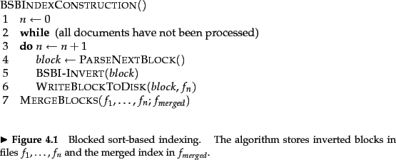
With main memory insufficient, we need to use an external sorting algorithm , that is, one that uses disk. For acceptable speed, the central requirement of such an algorithm is that it minimize the number of random disk seeks during sorting - sequential disk reads are far faster than seeks as we explained in Section 4.1 . One solution is the blocked sort-based indexing algorithm or BSBI in Figure 4.2 . BSBI (i) segments the collection into parts of equal size, (ii) sorts the termID-docID pairs of each part in memory, (iii) stores intermediate sorted results on disk, and (iv) merges all intermediate results into the final index.
The algorithm parses documents into termID-docID pairs and accumulates the pairs in memory until a block of a fixed size is full (PARSENEXTBLOCK in Figure 4.2 ). We choose the block size to fit comfortably into memory to permit a fast in-memory sort. The block is then inverted and written to disk. Inversion involves two steps. First, we sort the termID-docID pairs. Next, we collect all termID-docID pairs with the same termID into a postings list, where a posting is simply a docID. The result, an inverted index for the block we have just read, is then written to disk. Applying this to Reuters-RCV1 and assuming we can fit 10 million termID-docID pairs into memory, we end up with ten blocks, each an inverted index of one part of the collection.
![\includegraphics[width=11.5cm]{art/figure4.3.eps}](img189.png) Merging in blocked sort-based indexing.Two blocks (``postings lists to be merged'') are loaded from disk into
memory, merged in memory (``merged postings lists'') and written
back to disk. We show terms instead of termIDs for better readability.
Merging in blocked sort-based indexing.Two blocks (``postings lists to be merged'') are loaded from disk into
memory, merged in memory (``merged postings lists'') and written
back to disk. We show terms instead of termIDs for better readability.
In the final step, the algorithm simultaneously merges the
ten blocks into one large merged index. An example with two
blocks is shown in Figure 4.3 , where we use ![]() to
denote the
to
denote the ![]() document of the collection. To do
the merging, we open
all block files simultaneously, and maintain small read
buffers for the ten blocks we are reading and a write buffer for
the final merged index we are writing.
In each iteration, we select the lowest termID that has not
been processed yet using a priority queue or a similar data
structure. All postings lists for this termID are read
and merged, and the merged list is written back to disk.
Each read buffer is refilled from its file when
necessary.
document of the collection. To do
the merging, we open
all block files simultaneously, and maintain small read
buffers for the ten blocks we are reading and a write buffer for
the final merged index we are writing.
In each iteration, we select the lowest termID that has not
been processed yet using a priority queue or a similar data
structure. All postings lists for this termID are read
and merged, and the merged list is written back to disk.
Each read buffer is refilled from its file when
necessary.
How expensive is BSBI? Its time complexity
is
![]() because the step with the highest time
complexity is sorting and
because the step with the highest time
complexity is sorting and ![]() is an upper bound for the
number of items we must sort (i.e., the number of
termID-docID pairs). But the actual indexing time is
usually dominated by
the time it takes to parse the documents (PARSENEXTBLOCK) and to do the final merge (MERGEBLOCKS). Exercise 4.6 asks you to
compute the total index construction time for RCV1 that
includes these steps as well as inverting the blocks and writing them
to disk.
is an upper bound for the
number of items we must sort (i.e., the number of
termID-docID pairs). But the actual indexing time is
usually dominated by
the time it takes to parse the documents (PARSENEXTBLOCK) and to do the final merge (MERGEBLOCKS). Exercise 4.6 asks you to
compute the total index construction time for RCV1 that
includes these steps as well as inverting the blocks and writing them
to disk.
Notice that Reuters-RCV1 is not particularly large in an age when one or more GB of memory are standard on personal computers. With appropriate compression (Chapter 5 ), we could have created an inverted index for RCV1 in memory on a not overly beefy server. The techniques we have described are needed, however, for collections that are several orders of magnitude larger.
Exercises.
![\includegraphics[totalheight=5cm]{art/04-01.eps}](img187.png)